5.3.5 Dissociation Energy

The energy of the fragments in the laboratory frame of a moving molecule that dissociates can be calculated using a Galilei transformation [14]

$$E_{1/2}=\frac{1}{2}E_{0}+\frac{1}{2}E_{D}\pm \sqrt{E_{0}E_{D}}\cos {\alpha }\hspace {0.1cm},$$ (5.34)

where is the primary energy, the dissociation energy in the rest frame of the molecule, and the angle between the molecule axis and its velocity vector. The the energy spread measured can amount to substantial values due to the factor even tough might be only a few eV.

Assuming a uniform distribution of orientations of the molecules in space and a constant value of , the broadening of the energy distribution in the forward direction of the dissociated molecules can be estimated:

Using spherical coordinates with the particle moving in +z direction and an angle of the molecule axis to the z-axis, the energy of the particle in +z direction is given by Equation 5.34. With a uniform distribution of the molecule axis every direction has the same probability

$$p\left( \Omega \right) d\Omega =\frac{d\Omega }{4\pi }$$ (5.35)

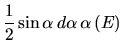
the solid angle may be expressed in terms of :

$$p\left( \alpha \right) d\alpha =\frac{2\pi \, \sin \alpha \, d\alpha }{4\pi }=\frac{1}{2}\sin \alpha \, d\alpha$$ (5.36)

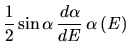
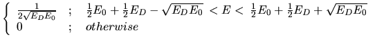
The probability for a particle to get the energy after dissociation is

$$p\left( E\right) dE = p\left( \alpha \right) d\alpha \, \cdot \, \alpha \left( E\right)$$ (5.37)

$$= \frac{1}{2}\sin \alpha \, d\alpha \, \alpha \left( E\right)$$ (5.38)

$$= \frac{1}{2}\sin \alpha \, dE\frac{d\alpha }{dE}\, \alpha \left( E\right)$$ (5.39)

is calculated using Equation 5.34 (only the forward accelerated particle is considered):

$$\alpha \left( E\right) =\arccos \left[ \frac{E\left( \alpha ... ...-\frac{1}{2}E_{0}-\frac{1}{2}E_{D}}{\sqrt{E_{0}E_{D}}}\right]$$ (5.40)

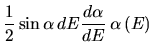
By substituting Equation 5.40 in Equation 5.39 and simplifying the energy distribution yields

$$p\left( E\right) = \frac{1}{2}\sin \alpha \, \frac{d\alpha }{dE}\, \alpha \left( E\right)$$ (5.41)

$$= \left\{ \begin{array}{ll} \frac{1}{2\sqrt{E_{D}E_{0}}} & ;\quad \... ...}+\frac{1}{2}E_{D}+\sqrt{E_{D}E_{0}}\\ 0 & ;\quad otherwise \end{array}\right.$$ (5.42)

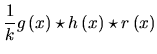
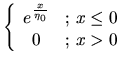
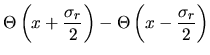
This simple model assuming an uniform distribution of the molecule axis yields a rectangular energy distribution in forward direction. By extending Equation 5.20 a new fit function was constructed consisting of a exponentional, a gaussian, and a rectangular part (Equations 5.43 to 5.46). is the Heaviside step function and denotes the full width of the rectangular part.

$$f_{m}\left( x\right) = \frac{1}{k}g\left( x\right) \star h\left( x\right) \star r\left( x\right)$$ (5.43)

$$g\left( x\right) = \left\{ \begin{array}{cr} e^{\frac{x}{\eta _{0}}} & ;\, x\leq 0\\ 0 & ;\, x>0 \end{array}\right.$$ (5.44)

$$h\left( x\right) = e^{-\frac{x^{2}}{2\sigma ^{2}_{g}}}$$ (5.45)

$$r\left( x\right) = \Theta \left( x+\frac{\sigma _{r}}{2}\right) -\Theta \left( x-\frac{\sigma _{r}}{2}\right)$$ (5.46)

The convolution was calculated numerically. Unfortunately this more physical fit function did not yield better fits than those calculated using Equation 5.31. The problem is that a convolution of a gaussian with a rectangular function of approximately the same width has a shape very similar to a single gaussian. This makes it difficult to separate (deconvolve) the rectangular part from the measured data especially if the gaussian part resulting from the energy distribution of the primary beam has approximately an energy width of the order of the to be separated rectangular function. Thus no further attempts were made to get the value of out of the time-of-flight data.